

WEMC Tech Blog #4: Calculating EU Country Averages With ERA5 and NUTS
As in previous blogs, this focuses on the Python programming language. For information on installing Python and packages, please see previous technical blogs #1 and #2.
This example will look at how to mask ERA5 data from the European region, downloaded from ECMWF Climate Data Store (CDS). The procedure heavily relies on functions provided by the scitools Iris package, although similar results could be obtained using a combination of packages like xarray and regionmask.
Import the following packages:
[pastacode lang=”python” manual=”%23%20import%20packages%0Aimport%20iris%0Aimport%20geopandas%20as%20gpd%0Aimport%20numpy%20as%20np%0Aimport%20matplotlib.pyplot%20as%20plt%0Aimport%20cartopy.crs%20as%20ccrs%0Aimport%20iris.plot%20as%20iplt%0Aimport%20iris.quickplot%20as%20qplt%0Aimport%20iris.pandas%0Aimport%20os” message=”” highlight=”” provider=”manual”/]Read in the NUTS (Nomenclature of Territorial Units for Statistics) shapefile using geopandas. NUTS shapefiles are obtained from eurostat, who provide various resolutions and formats to use in your code. For this example, a scale 1:20 Million is used, in the SHP (shapefile) format. Level 0 is the lowest resolution and is a collection of geometric polygons at country level.
[pastacode lang=”python” manual=”%23%20read%20the%20NUTS%20shapefile%20and%20extract%20the%20polygons%20for%20a%20individual%20countries%0Anuts%3Dgpd.read_file(‘ref-nuts-2016-20m.shp%2FNUTS_RG_20M_2016_4258_LEVL_0.shp’)” message=”” highlight=”” provider=”manual”/]A quick check of the NUTS shapefile reveals the geometry values, with some associated identifiers.
[pastacode lang=”python” manual=”nuts” message=”” highlight=”” provider=”manual”/]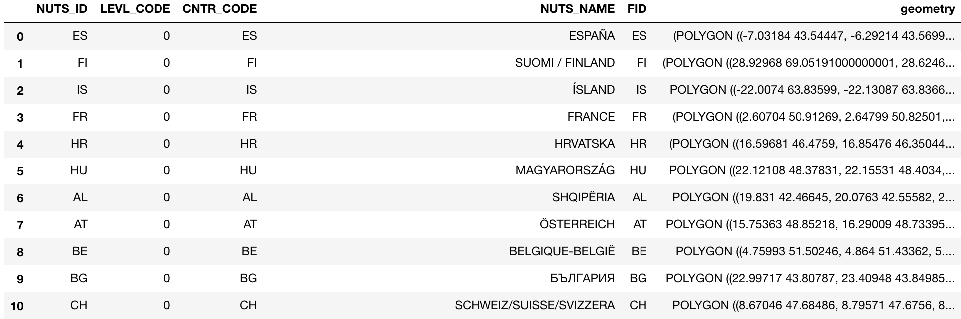
Select a country by its abbreviation (aka ‘NUTS_ID’). For example, ‘FR’ will select the France shapefile.
[pastacode lang=”python” manual=”%23%20set%20country%20by%20NUTS_ID%0Acountry%20%3D%20nuts%5Bnuts%5B’NUTS_ID’%5D%20%3D%3D%20’FR’%5D” message=”” highlight=”” provider=”manual”/]Load in a NetCDF file using Iris. Iris has many built in functions for dealing with NetCDF. As discussed in previous blogs, NetCDF files are a file format for storing multidimensional data. Iris represents this data as ‘cubes’, a convenient way to manipulate NetCDF data, whilst keeping things cf compliant. Here, a NetCDF containing 1 year (2000) of hourly 2 metre temperature, covering the EU region, is loaded.
[pastacode lang=”python” manual=”%23%20get%20the%20latitude-longitude%20grid%20from%20netcdf%20file%0Acubelist%3Diris.load(‘ecmwf_era5_analysis_S200001010000_E200012312300_1hr_EU1_025d_2m_t2m_noc_org.nc’)%0Acube%3Dcubelist%5B0%5D%0Acube%3Dcube.intersection(longitude%3D(-180%2C%20180))” message=”” highlight=”” provider=”manual”/]Once loaded, a quick check of the cube shows it has three dimensions; time, latitude and longitude. With the variable 2 metre temperature (K).
[pastacode lang=”python” manual=”cube” message=”” highlight=”” provider=”manual”/]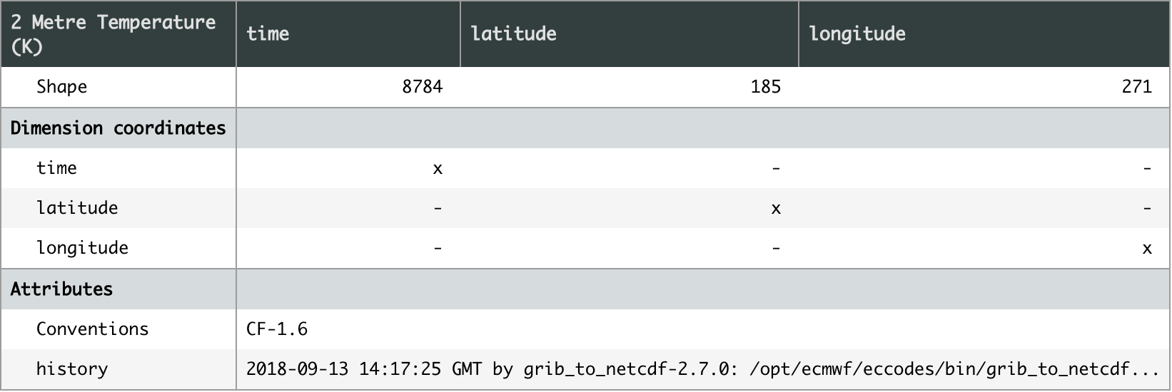
Next, create a function to check whether the data is within the boundaries of the shapefile. Surprisingly, Iris does not have a function to do this out-of-the-box, so I borrowed this good example from a post on stack overflow (credit to user DPeterK).
[pastacode lang=”python” manual=”%23%20function%20to%20check%20whether%20data%20is%20within%20shapefile%20-%20source%3A%20http%3A%2F%2Fbit.ly%2F2pKXnWa%0A%0Adef%20geom_to_masked_cube(cube%2C%20geometry%2C%20x_coord%2C%20y_coord%2C%0A%20%20%20%20%20%20%20%20%20%20%20%20%20%20%20%20%20%20%20%20%20%20%20%20mask_excludes%3DFalse)%3A%0A%20%20%20%20%22%22%22%0A%20%20%20%20Convert%20a%20shapefile%20geometry%20into%20a%20mask%20for%20a%20cube’s%20data.%0A%0A%20%20%20%20Args%3A%0A%0A%20%20%20%20*%20cube%3A%0A%20%20%20%20%20%20%20%20The%20cube%20to%20mask.%0A%20%20%20%20*%20geometry%3A%0A%20%20%20%20%20%20%20%20A%20geometry%20from%20a%20shapefile%20to%20define%20a%20mask.%0A%20%20%20%20*%20x_coord%3A%20(str%20or%20coord)%0A%20%20%20%20%20%20%20%20A%20reference%20to%20a%20coord%20describing%20the%20cube’s%20x-axis.%0A%20%20%20%20*%20y_coord%3A%20(str%20or%20coord)%0A%20%20%20%20%20%20%20%20A%20reference%20to%20a%20coord%20describing%20the%20cube’s%20y-axis.%0A%0A%20%20%20%20Kwargs%3A%0A%0A%20%20%20%20*%20mask_excludes%3A%20(bool%2C%20default%20False)%0A%20%20%20%20%20%20%20%20If%20False%2C%20the%20mask%20will%20exclude%20the%20area%20of%20the%20geometry%20from%20the%0A%20%20%20%20%20%20%20%20cube’s%20data.%20If%20True%2C%20the%20mask%20will%20include%20*only*%20the%20area%20of%20the%0A%20%20%20%20%20%20%20%20geometry%20in%20the%20cube’s%20data.%0A%0A%20%20%20%20..%20note%3A%3A%0A%20%20%20%20%20%20%20%20This%20function%20does%20*not*%20preserve%20lazy%20cube%20data.%0A%0A%20%20%20%20%22%22%22%0A%20%20%20%20%23%20Get%20horizontal%20coords%20for%20masking%20purposes.%0A%20%20%20%20lats%20%3D%20cube.coord(y_coord).points%0A%20%20%20%20lons%20%3D%20cube.coord(x_coord).points%0A%20%20%20%20lon2d%2C%20lat2d%20%3D%20np.meshgrid(lons%2Clats)%0A%0A%20%20%20%20%23%20Reshape%20to%201D%20for%20easier%20iteration.%0A%20%20%20%20lon2%20%3D%20lon2d.reshape(-1)%0A%20%20%20%20lat2%20%3D%20lat2d.reshape(-1)%0A%0A%20%20%20%20mask%20%3D%20%5B%5D%0A%20%20%20%20%23%20Iterate%20through%20all%20horizontal%20points%20in%20cube%2C%20and%0A%20%20%20%20%23%20check%20for%20containment%20within%20the%20specified%20geometry.%0A%20%20%20%20for%20lat%2C%20lon%20in%20zip(lat2%2C%20lon2)%3A%0A%20%20%20%20%20%20%20%20this_point%20%3D%20gpd.geoseries.Point(lon%2C%20lat)%0A%20%20%20%20%20%20%20%20res%20%3D%20geometry.contains(this_point)%0A%20%20%20%20%20%20%20%20mask.append(res.values%5B0%5D)%0A%0A%20%20%20%20mask%20%3D%20np.array(mask).reshape(lon2d.shape)%0A%20%20%20%20if%20mask_excludes%3A%0A%20%20%20%20%20%20%20%20%23%20Invert%20the%20mask%20if%20we%20want%20to%20include%20the%20geometry’s%20area.%0A%20%20%20%20%20%20%20%20mask%20%3D%20~mask%0A%20%20%20%20%23%20Make%20sure%20the%20mask%20is%20the%20same%20shape%20as%20the%20cube.%0A%20%20%20%20dim_map%20%3D%20(cube.coord_dims(y_coord)%5B0%5D%2C%0A%20%20%20%20%20%20%20%20%20%20%20%20%20%20%20cube.coord_dims(x_coord)%5B0%5D)%0A%20%20%20%20cube_mask%20%3D%20iris.util.broadcast_to_shape(mask%2C%20cube.shape%2C%20dim_map)%0A%0A%20%20%20%20%23%20Apply%20the%20mask%20to%20the%20cube’s%20data.%0A%20%20%20%20data%20%3D%20cube.data%0A%20%20%20%20masked_data%20%3D%20np.ma.masked_array(data%2C%20cube_mask)%0A%20%20%20%20cube.data%20%3D%20masked_data%0A%20%20%20%20return%20cube” message=”” highlight=”” provider=”manual”/]The function can now be applied to the cube, in this case checking whether the data is within the France polygon.
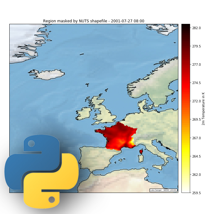
[pastacode lang=”python” manual=”%23%20apply%20the%20geom_to_masked_cube%20function%0Ageometry%20%3D%20country%0Amasked_cube%20%3D%20geom_to_masked_cube(cube%2C%20geometry%2C%20’longitude’%2C%20’latitude’%2C%20mask_excludes%3DTrue)” message=”” highlight=”” provider=”manual”/]Plotting an individual time slice from ‘masked_cube’, reveals the data is now successfully masked to the France region.
[pastacode lang=”python” manual=”%23%20plot%20to%20check%20area%20masking%20is%20correct%0Aplt.figure(figsize%3D(20%2C%2010)%2C)%0Aax%20%3D%20plt.axes(projection%3Dccrs.PlateCarree())%0A%0A%23%20pick%20time%20slice%20and%20draw%20the%20contour%20with%20100%20levels%20%2B%20select%20appropriate%20cmap.%0Aq%20%3D%20iris.plot.contourf(masked_cube%5B5000%5D%2C%20100%2C%20cmap%3D’hot_r’)%0A%0A%23%20add%20colour%20bar%20w%2Flabel%0Acb%20%3D%20plt.colorbar()%0Acb.set_label(‘2m%20Temperature%20in%20K’)%0A%0A%23%20add%20coastlines%20to%20the%20map%20created%20by%20contourf.%0Aax.coastlines(resolution%3D’50m’)%0A%0A%23%20add%20stock%20background%20image%0Aax.stock_img()%0A%0A%23%20add%20title%0Aplt.title(‘Region%20masked%20by%20NUTS%20shapefile%20-%202001-07-27%2008%3A00’)%0A%0A%23%20Add%20a%20citation%20to%20the%20plot.%0Aiplt.citation(‘Luke%20Sanger%20-%20WEMC%20(2018)’)%0A%0A%23%20set%20map%20limits%20to%20show%20only%20EU%0Aax.set_extent(%5B-30.0%2C%2020.0%2C%2030.0%2C%2080.0%5D%2C%20ccrs.PlateCarree())%0A%0A%23%20show%20plot%0Aplt.show()” message=”” highlight=”” provider=”manual”/]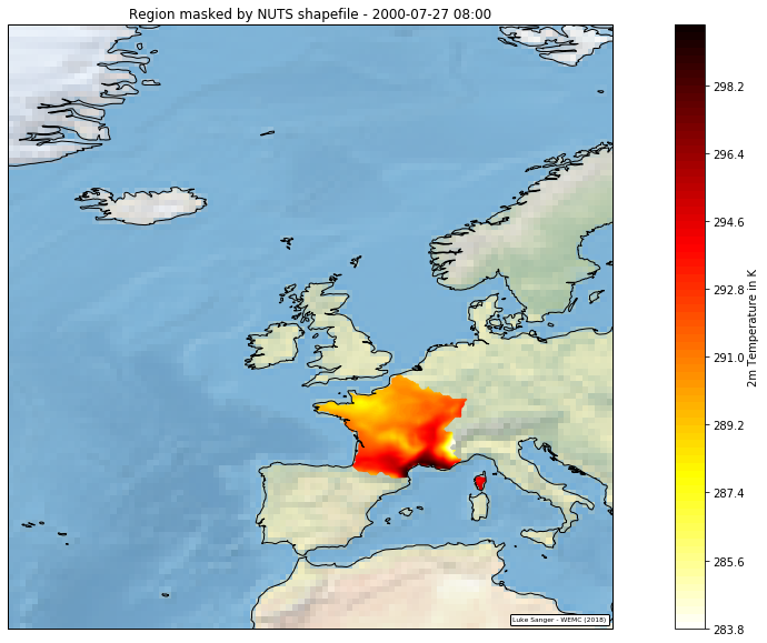
Before getting the area average, it’s important to note the current grid is a euclidean space, a flat grid of equal dimensions. To account for the curvature of the earth, create area weights utilising the Iris ‘cosine_latitude_weights’ function.
[pastacode lang=”python” manual=”%23%20use%20iris%20function%20to%20get%20area%20weights%0Agrid_areas%20%3D%20iris.analysis.cartography.cosine_latitude_weights(masked_cube)” message=”” highlight=”” provider=”manual”/]These weights can be used in conjunction with the ‘iris_analysis_MEAN’ function to collapse the cube into a 1-dimensional array.
[pastacode lang=”python” manual=”new_cube%20%3D%20masked_cube.collapsed(%5B’latitude’%2C’longitude’%5D%2C%20iris.analysis.MEAN%2C%20weights%3Dgrid_areas)” message=”” highlight=”” provider=”manual”/]Finally, in order to output this into a .csv file. First convert to a pandas series, then save as csv.
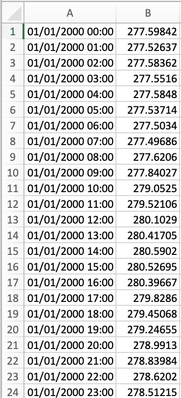
[pastacode lang=”python” manual=”%23%20convert%20to%20pandas%20series%20%0Adfs%20%3D%20iris.pandas.as_series(new_cube)%0A%0A%23%20save%20as%20csv%0Adfs.to_csv(‘csv_name’)” message=”” highlight=”” provider=”manual”/]Opening the .csv file should produce a dataset containing the time series and the area averages for that country.
In the future I will revisit this topic with a follow up blog looking at applying a land-sea mask to the dataset. This improves accuracy where land sea boundaries occupy grid areas and applies weights based on this.
An example dataset can be downloaded here
Complete ipython notebook code can be found on my github page here
by Luke Sanger (WEMC Data Engineer, 2018)

