

WEMC TECH BLOG #3: ERA5 10m/100m Analysis
We wanted to see if we could improve on the standard power law coefficient (1.389495) for calculating 100m wind speed from 10m data. The currently available ten years of ERA5 U and V netCDF wind components from CDS were concatenated, then calculated for wind speed using CDO; a handy collection of command-line operators to manipulate and analyse climate and numerical weather prediction data:
[pastacode lang=”bash” manual=”cdo%20sqrt%20-add%20-sqr%2010Uall.nc%20-sqr%2010Vall.nc%2010wind.nc” message=”” highlight=”” provider=”manual”/] [pastacode lang=”bash” manual=”cdo%20sqrt%20-add%20-sqr%20100Uall.nc%20-sqr%20100Vall.nc%20100wind.nc” message=”” highlight=”” provider=”manual”/]The coefficient dataset was calculated with CDO, by dividing 100m by 10m datasets:
[pastacode lang=”bash” manual=”cdo%20div%20100wind.nc%2010wind.nc%20coef.nc” message=”” highlight=”” provider=”manual”/]The mean coefficient for the whole domain is 1.448035, slightly higher than the standard coefficient, taking it further away from the newly available ERA5 100m forecast data. The average standard deviation is 0.816657.
The ratio as a function of the geographical location was then plotted in Python, using matplotlib package’s plot.imshow() method.
First load the necessary python packages:
[pastacode lang=”python” manual=”%23%20importing%20of%20NetCDF%20files%0Aimport%20netCDF4%0A%0A%23%20plotting%20and%20data%20visualisations%0Afrom%20matplotlib%20import%20pyplot%20as%20plt%0A%0A%23%20n-dimensional%20arrays%0Aimport%20numpy%20as%20np%0A%0A%23%20high%20level%20functions%20for%20working%20with%20NetCDF%20files%0Aimport%20xarray%20as%20xr” message=”” highlight=”” provider=”manual”/]
Import the pre-calculated coefficient dataset:
[pastacode lang=”python” manual=”%23%20load%20NetCDF%20file%20into%20variable%20-%20using%20xarray%20open%20dataset%20function%0A%0Acoef%20%3D%20xr.open_dataset(‘%2FUsers%2Fuser%2FDocuments%2FERA5%2Fyearly_complete%2Fallyears%2Fcoef.nc’)” message=”” highlight=”” provider=”manual”/]
Calculate the mean average using the numpy mean method:
[pastacode lang=”python” manual=”%23%20calculate%20mean%20over%2010%20year%20dataset%0At%20%3D%20coef.mean(‘time’)” message=”” highlight=”” provider=”manual”/]
Finally, plot the total wind speed average using matplotlib imshow() method, note interpolation is set to ‘none’, this can be changed to apply various smoothing algorithms:
[pastacode lang=”python” manual=”%23%20plot%20mean%20average%20of%20full%2010%20years%0At.uv100.plot.imshow(figsize%3D(15%2C10)%2Cinterpolation%3D’none’)” message=”” highlight=”” provider=”manual”/]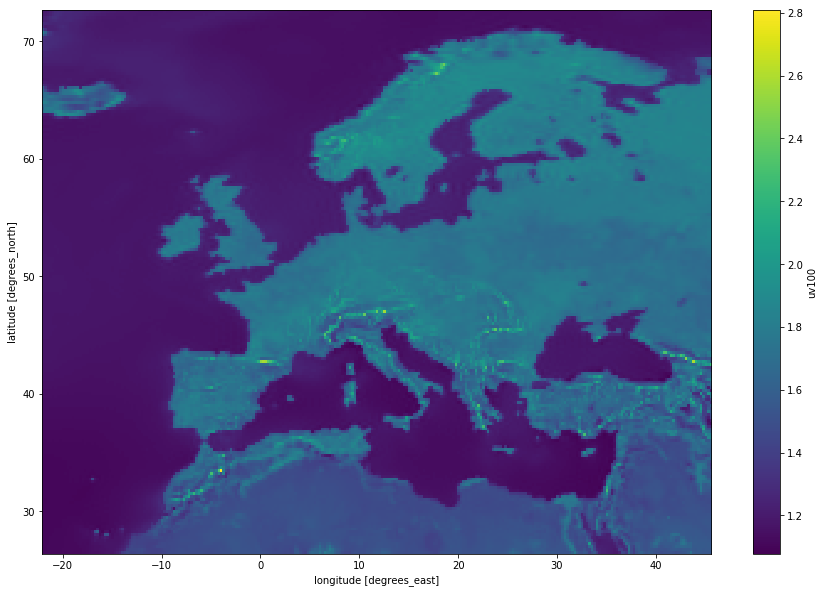
Ratio 100m divided by 10m for ERA5 averaged over the period 2008-2017
Next we can check the standard deviation over this time period:
[pastacode lang=”python” manual=”%23%20calculate%20standard%20deviation%20over%20full%2010%20years%0Astd%20%3D%20coef.std(‘time’)” message=”” highlight=”” provider=”manual”/]
For this plot, the colour map (cmap=’terrain’) was adjusted to highlight the variation:
[pastacode lang=”python” manual=”%23%20plot%20standard%20deviation%20of%20full%2010%20years%0Astd.uv100.plot.imshow(figsize%3D(15%2C10)%2Cinterpolation%3D’none’%2Ccmap%3D’terrain’)” message=”” highlight=”” provider=”manual”/]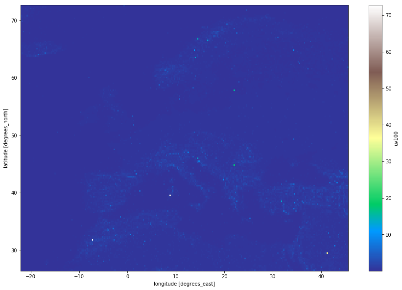
Standard Deviation of the ratio 100m divided by 10m for ERA5 over the period 2008-2017
This indicates that a geographically-dependent coefficient would better reproduce the 100 m wind, when only 10 m is available.
by Luke Sanger (WEMC, 2018)


